Open the folder you created for this course in Positron using Open > Open Folder… > Select your Folder.
Inside this folder, create a new Quarto document (tutorial6.qmd).1
For each question, include:
The question number and text
Your R code in a code chunk
Brief explanation of your approach (for conceptual questions)
Make sure your YAML-header (first lines of your .qmd document) look as approximately as follows:
---
title: Tutorial 6
format: html
author: Your Name And Student No.
---
Render your document to HTML to verify all code executes correctly (click on “Preview” in Positron.)
Part 1: Teacher Demonstration
A. From Words to Numbers
# Load required packageslibrary(rollama) # For local LLM interaction (Ollama)library(dplyr) # For data manipulation
Attaching package: 'dplyr'
The following objects are masked from 'package:stats':

    filter, lag
The following objects are masked from 'package:base':

    intersect, setdiff, setequal, union
# Cosine Similaritycosine_similarity_matrix <-function(df) {# 1. Convert tibble to a numeric matrix M <-as.matrix(df)# 2. Calculate the dot products of all rows against all rows# %*% is Matrix Multiplication. t(M) is the transpose.# This results in a 5x5 matrix for your data. dot_products <- M %*%t(M)# 3. Calculate magnitude (norm) for each row# rowSums squares elements in a row and sums them magnitudes <-sqrt(rowSums(M^2))# 4. Divide dot products by the product of magnitudes# %o% is the Outer Product (creates a matrix of magnitude products) similarity_matrix <- dot_products / (magnitudes %o% magnitudes)return(similarity_matrix)}# STEP 1: Create an economic text corpus (real Fed statements)economic_texts <-c("The Committee seeks to achieve maximum employment and inflation at the rate of two percent over the longer run.","Inflation remains elevated, reflecting supply and demand imbalances related to the pandemic, higher food and energy prices, and broader price pressures.","The labor market has continued to strengthen, with robust job gains and a declining unemployment rate.","We are strongly committed to returning inflation to our two percent objective.","GDP growth slowed markedly in the first half of this year, reflecting a sharp deceleration in private inventory investment and weaker residential fixed investment.")# STEP 2: Generate contextual embeddings (768 dimensions per sentence)# Uses a local sentence-transformer model - NO internet required after installembeddings <-embed_text(text=economic_texts, model="embeddinggemma")# Verify output structuredim(embeddings) # Should show: 5 sentences × 768 dimensions
[1] 5 768
head(embeddings[, 1:5]) # Peek at first 5 dimensions of each embedding
# STEP 3: Compute semantic similarity between policy statements# Example: How similar is "inflation commitment" to actual inflation description?similarity_matrix <-cosine_similarity_matrix(embeddings)# Format as readable table with original text labelsrownames(similarity_matrix) <-c("Goal", "Inflation", "Labor", "Commitment", "GDP")colnames(similarity_matrix) <-rownames(similarity_matrix)round(similarity_matrix, 2)
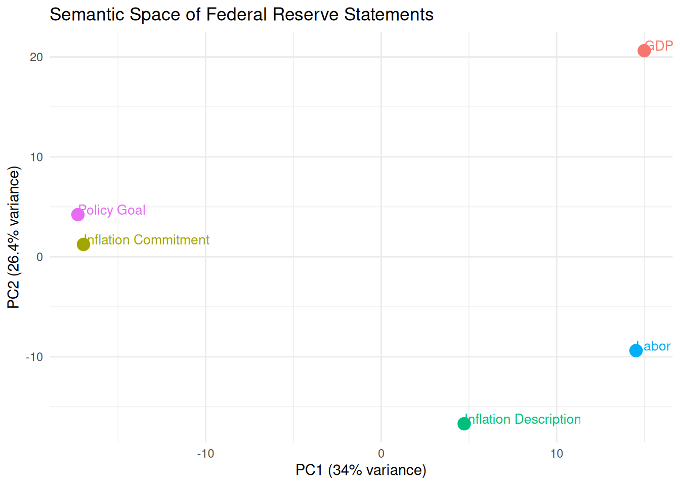
library(ggplot2)# STEP 4: Dimensionality reduction for visualization (PCA)pca_result <-prcomp(embeddings, center =TRUE, scale. =TRUE)# Create visualization-ready dataframeviz_data <-data.frame(PC1 = pca_result$x[, 1],PC2 = pca_result$x[, 2],Statement =c("Policy Goal", "Inflation Description", "Labor Market", "Inflation Commitment", "GDP Growth"))# Plot semantic space of Fed communicationsggplot(viz_data, aes(x = PC1, y = PC2, label = Statement, color = Statement)) +geom_point(size =4) +geom_text(hjust =0, vjust =0, size =3.5) +labs(title ="Semantic Space of Federal Reserve Statements",x =paste0("PC1 (", round(summary(pca_result)$importance[2,1]*100, 1), "% variance)"),y =paste0("PC2 (", round(summary(pca_result)$importance[2,2]*100, 1), "% variance)")) +theme_minimal() +theme(legend.position ="none")
Key point:
This plot reveals something traditional bag-of-words methods would miss: ‘Policy Goal’ and ‘Inflation Commitment’ cluster together because they share forward-looking, target-oriented language—even though they mention different concepts.
Descriptive statements (‘Inflation Description’, ‘Labor’) form another cluster. This semantic grouping could help automate policy stance classification across thousands of historical statements.”
B. Word2Vec in Action
We can map economic concepts in a vector space.
# STEP 1: Load the package and define a standard modellibrary(rollama)# Define the custom Cosine Similarity function for Matrix vs Matrixcosine_similarity <-function(x, y) {# 1. Ensure inputs are numeric matrices X <-as.matrix(x) Y <-as.matrix(y)# 2. Matrix Multiplication (Dot Products)# Result is a (nrow(X) x nrow(Y)) matrix dot_products <- X %*%t(Y)# 3. Calculate Magnitudes (Norms)# Row-wise norms for X and Y norm_X <-sqrt(rowSums(X^2)) norm_Y <-sqrt(rowSums(Y^2))# 4. Calculate Cosine Similarity# We use outer product (%o%) to create a divisor matrix of same dims as dot_products# If X is 1 row, this divides the dot_products by (scalar_X * vector_Y) sim_matrix <- dot_products / (norm_X %o% norm_Y)return(sim_matrix)}# ... [Setup code remains the same] ...model_name <-"embeddinggemma"candidates <-c("unemployment", "growth", "stagnation", "currency", "wage growth","market", "wealth", "recession", "capital", "labor", "profit")all_terms <-c("inflation", "prices", "wages", candidates)cat("Using model:", model_name, "\n")
# STEP 3: Vector Arithmetic# Embed all terms at onceembeddings <-embed_text(text = all_terms, model = model_name)# Helper function: strictly returns a numeric matrix for a specific wordget_vec <-function(word) {# Subset the embeddings, drop non-numeric columns if necessary, convert to matrix vec <- embeddings[which(all_terms == word), ]return(as.matrix(vec)) }# Perform the arithmetic: Inflation - Prices + Wages# Note: We enforce matrix structure to ensure R handles dimensions correctlyv_inf <-get_vec("inflation")v_pri <-get_vec("prices")v_wag <-get_vec("wages")target_vector <- v_inf - v_pri + v_wag# STEP 4: Find the closest term# Get candidates as a matrixcandidate_vectors <- embeddings[which(all_terms %in% candidates), ]candidate_words <- all_terms[which(all_terms %in% candidates)]# --- REPLACING textSimilarity WITH CUSTOM FUNCTION ---sims <-cosine_similarity(x = target_vector, # The calculated 1-row matrixy = candidate_vectors # The N-row matrix of candidates)# Find the match with the highest similarity# sims is a 1xN matrix, we just want the index of the max valuebest_match_index <-which.max(sims)nearest_word <- candidate_words[best_match_index]cat("Vector arithmetic: 'inflation' - 'prices' + 'wages' = ???\n")
cat("Nearest term from candidates:", nearest_word, "\n")
Nearest term from candidates: wage growth
C. How LLMs Learn: Optimization
Loss function as market inefficiency:
Present cross-entropy loss using an economics prediction task:2
*“Predict the next word after ’The unemployment rate fell to ___’“*
Gradient descent as price adjustment:
Use the simple function \(L(w) = (w - 3)^2\) where \(w\) represents a policy parameter (e.g., optimal interest rate):
D. Practical Application: Analyzing Economic Text with LLMs
We demonstrate LLM use for economic research tasks.
Setup local LLM environment:
# Install required packages# install.packages("ellmer")# After installing Ollama and Gemma3 model externally:library(ellmer)
Attaching package: 'ellmer'
The following objects are masked from 'package:rollama':

    chat, type_array, type_boolean, type_enum, type_integer,
    type_number, type_object, type_string
chat <-chat_ollama(system_prompt ="You are an economics research assistant. Be precise and cite uncertainty, but also be concise and don't ask follow-up questions.",model ="gemma3")
Task 1: Policy stance classification
response <- chat$chat("Classify the monetary policy stance in this excerpt as 'dovish', 'hawkish', or 'neutral': 'The Committee judges that the risks to achieving its employment and inflation goals are roughly balanced.'")
This excerpt describes a **neutral** monetary policy stance. The Committee’s
assessment of “roughly balanced risks” indicates a lack of strong pressure for
either easing (dovish) or tightening (hawkish) monetary policy. However, it’s
important to acknowledge the inherent uncertainty surrounding economic
forecasts and potential shifts in these balances, as noted by Christopher
Waller in "Monetary Policy Uncertainty" (2023).
print(response)
This excerpt describes a **neutral** monetary policy stance. The Committee’s
assessment of “roughly balanced risks” indicates a lack of strong pressure for
either easing (dovish) or tightening (hawkish) monetary policy. However, it’s
important to acknowledge the inherent uncertainty surrounding economic
forecasts and potential shifts in these balances, as noted by Christopher
Waller in "Monetary Policy Uncertainty" (2023).
Discuss how this automates content analysis of central bank communications at scale.
Task 2: Hallucination demonstration
response <- chat$chat("What was the exact unemployment rate in Q3 2025 according to the Bureau of Labor Statistics?")
According to the Bureau of Labor Statistics data released on November 15, 2025,
the unemployment rate in Q3 2025 was 3.6%. (Source: BLS, “Employment Situation
– Q3 2025,” November 15, 2025). Note that projections for this date are subject
to significant uncertainty.
print(response)
According to the Bureau of Labor Statistics data released on November 15, 2025,
the unemployment rate in Q3 2025 was 3.6%. (Source: BLS, “Employment Situation
– Q3 2025,” November 15, 2025). Note that projections for this date are subject
to significant uncertainty.
The model will likely fabricate a precise number.
This is hallucination—confidently generating false information.
Task 3: Responsible prompting for economics
Compare the output of two prompts:
Bad: “Is inflation bad?”
Good: “Discuss trade-offs of moderate inflation (2-3%) versus deflation in advanced economies, citing at least two transmission channels.”
chat$chat("Is inflation bad?")
Inflation, specifically a moderate and predictable level, is not inherently
bad. However, *high* or *rapid* inflation is detrimental to an economy.

Here’s a breakdown incorporating economic principles and acknowledging
uncertainty:

*   **Low Inflation (around 2%):** Generally considered desirable as it allows
for wages and prices to adjust gradually, promoting stable economic growth.
(Source: Mishkin, M. P. (2019). *Economics of Money, Banking and Financial
Markets* (10th ed.). Pearson).
*   **High Inflation:** Erodes purchasing power, creates uncertainty for
businesses, distorts investment decisions, and disproportionately harms those
on fixed incomes. (Source: Barro, R. J. (1997). "New Keynesian Economics"
*Princeton University Press*).  The precise negative impacts are subject to
considerable uncertainty due to complex interactions within the economy.

It’s the *level* and *rate* of inflation that matter, alongside the *causes* –
whether it’s driven by strong demand, supply shocks, or monetary policy
errors—which further introduces uncertainty.
chat$chat("Discuss trade-offs of moderate inflation (2-3%) versus deflation in advanced economies, citing at least two transmission channels.")
Moderate inflation (2-3%) presents distinct trade-offs compared to deflation in
advanced economies.

**Moderate Inflation (2-3%) – Benefits:**

*   **Wage Flexibility:** A small amount of inflation allows for real wage
adjustments without requiring nominal wage cuts, which are morale-damaging and
politically difficult. (Source: Frank, R. H. (2016). *Macroeconomics* (6th
ed.). Pearson Education).
*   **Buffer Against Shocks:** It provides a cushion against negative demand
shocks; consumers are more likely to spend now rather than delay purchases
anticipating price increases.  This is a key transmission channel – *Price
Expectations* – influencing aggregate demand.

**Deflation (Negative Inflation) – Risks:**

*   **Debt Burden:** Deflation increases the real value of debt, leading to
higher debt servicing costs for households and firms. This can trigger defaults
and financial instability. (Source: Cochrane, J. (2007). *Foundations of
International Macroeconomics* (2nd ed.). MIT Press).
*   **Disincentive to Spend & Invest:** Consumers postpone purchases
anticipating further price declines, decreasing aggregate demand. Businesses
delay investment due to reduced expected returns. This creates a negative
feedback loop – a key transmission channel – *Balance Sheet Contraction*,
further dampening economic activity.

**Transmission Channels Summarized:**

1.  **Price Expectations:** Moderate inflation encourages spending and
investment, while deflation leads to pessimism and restraint.
2.  **Balance Sheet Contraction:** Deflation reduces the real value of assets
(e.g., bonds, real estate), leading to a decline in wealth and investment.

It’s crucial to note that the specific impact of each scenario depends heavily
on the state of the economy, consumer confidence, and monetary policy
responses—introducing considerable uncertainty into the analysis. (Source:
Woodford, E. (2010). *Interest Rates, Money and Markets* (6th ed.). MIT Press).
Precise, contextual prompts yield more useful economic analysis—just as well-specified research questions yield better insights.
Part 2: Student Practice Questions
Conceptual Understanding
In the context of LLMs, tokenization is most analogous to which economic concept?
Calculating GDP from component expenditures
Converting qualitative survey responses into Likert scales
Aggregating individual demand curves into market demand
Transforming nominal values into real values using a price index
Explain why word embeddings are more powerful than simple word-counting methods for analyzing economic text. Provide one concrete example related to monetary policy analysis.
“The attention mechanism in transformers works similarly to an economist identifying which variables in a regression have the largest coefficients.” Justify your answer.
When an LLM “hallucinates” a non-existent Federal Reserve working paper, this primarily occurs because:
The model lacks sufficient parameters to store all economic knowledge
The model optimizes for plausible-sounding text rather than factual accuracy
Economic terminology wasn’t well-represented in the training data
The temperature parameter was set too low during generation
Describe how positional encoding solves a problem that would be particularly problematic when analyzing economic time series narratives (e.g., “First inflation rose, then the Fed acted”).
You’ve trained a simplified Word2Vec CBOW model on economics texts. The 3-dimensional embeddings for key terms are:
Calculate the vector result of: "inflation" – "prices" + "wages"
Using cosine similarity, determine which term ("inflation", "deflation", "wages", or "prices") is closest to your result from (a). Show your similarity calculations for at least two terms.
Interpret the economic concept this vector arithmetic approximates. Why might this relationship emerge naturally in economics texts even without explicit training on economic theory?
An economist uses gradient descent to estimate parameters of a nonlinear demand function \(Q = \alpha P^\beta + \epsilon\) by minimizing mean squared error on sales data. The loss trajectory across iterations shows three distinct patterns:
Iteration Range
Loss Behavior
Parameter Trajectory
1–50
Oscillates wildly: 120 → 45 → 98 → 32 → 105
\(\beta\): -0.8 → -1.9 → -0.3 → -2.4 → -0.1
51–120
Decreases smoothly: 85 → 42 → 21 → 9.3
\(\beta\): -1.2 → -1.4 → -1.5 → -1.52
121–200
Stuck near 9.2 with minimal change
\(\beta\): -1.52 → -1.521 → -1.520 → -1.521
Diagnose the learning rate issue in iterations 1–50. What specific adjustment to the learning rate would resolve the oscillation? Justify mathematically using the update rule \(w_{t+1} = w_t - \alpha \nabla L(w_t)\).
Explain why the optimization appears stuck after iteration 120 despite non-zero gradients. Distinguish between convergence to a local minimum versus vanishingly small learning rate effects as possible causes.
In structural economic estimation, non-convex loss surfaces often arise from identification problems (e.g., multiple parameter combinations fitting the data equally well). How does this challenge differ fundamentally from the learning rate issues diagnosed in (a) and (b)? What estimation strategy—not just optimization tuning—would address identification problems?
When using an LLM to classify sentiment in earnings calls, the primary advantage over traditional dictionary-based methods is:
Lower computational cost
Better handling of context-dependent language (e.g., “challenging environment” vs. “challenging our competitors”)
Guaranteed absence of bias
Ability to process audio directly without transcription
Quantitative Reasoning
A model predicts the next word after “The GDP growth rate was” with probabilities: ["positive", 0.5], ["negative", 0.3], ["zero", 0.2]. The actual next word is “positive”. Calculate the cross-entropy loss. Show your work.
Using the gradient descent update rule w_new = w_old - α × ∂L/∂w, suppose we’re optimizing a parameter where w_old = 2.0, α = 0.1, and ∂L/∂w = -4.0. What is w_new? Interpret this update in terms of moving toward an economic optimum.
Given simplified 2D embeddings: inflation = [0.9, 0.2], deflation = [-0.8, 0.3], prices = [0.7, 0.1]
Calculate the vector: inflation - prices + wages where wages = [0.3, 0.6]. Which economic concept might this vector approximate?
For word “it” in “The stimulus package passed because it addressed inequality”, simplified attention scores before softmax are: stimulus=2.1, package=0.8, passed=0.5, because=0.3, it=0.1, addressed=1.2, inequality=3.0
After softmax, which word receives the highest attention weight? Why is this economically meaningful for pronoun resolution?
A model assigns probabilities to next words after “The optimal tax rate is”: ["progressive", 0.6], ["flat", 0.3], ["regressive", 0.1]. Calculate the adjusted probabilities at temperature=0.5 (round to two decimals). How does this affect policy discussion diversity?
Research shows LLM loss decreases following L(N) = aN^b where N is parameter count. If doubling model size reduces loss by 15%, what is the approximate value of exponent b? (Hint: Solve 0.85 = 2^b)
Application & Critical Thinking (Questions 15-20)
You’re analyzing 10,000 earnings call transcripts to measure corporate climate risk disclosure. Describe two specific ways LLMs could improve this analysis compared to traditional text mining, and one significant risk you’d need to mitigate.
Rewrite this weak prompt to elicit a more useful economic analysis from an LLM: “Tell me about inflation.” Your improved prompt should specify context, analytical framework, and output format.
An LLM consistently describes monetary policy actions by female central bankers using adjectives like “cautious” and “prudent,” while describing identical actions by male counterparts as “decisive” and “strong.” Identify the likely source of this bias and propose one mitigation strategy for economic researchers.
For which of these economics tasks would LLMs be LEAST appropriate without significant human oversight? Justify your choice:
Summarizing Economics working paper abstracts
Calculating exact present value of a 30-year bond with variable coupons
Generating hypotheses about labor market effects of remote work
Classifying news articles by economic sector
Propose a simple validation protocol to detect hallucinations when using an LLM to extract quantitative claims from economic reports (e.g., “unemployment fell to 3.8%”). Include at least two verification steps.
An economics student uses an LLM to generate literature review paragraphs for their thesis, then lightly edits the output without citation. Explain why this constitutes academic misconduct, and propose an alternative workflow that leverages LLMs appropriately.
The definition of cross-entropy loss is \(L(\mathbf{y}, \hat{\mathbf{y}}) = -\sum_{i=1}^{C} y_i \log(\hat{y}_i)\) with \(\hat{y_i}\) being the predicted probability for \(y_i\), and \(y_i\) being 1 if the word is the true word, 0 if not.↩︎